Case study 1

To investigate the role of large and megaherbivores in the Serengeti, we removed endothermic herbivores with a body mass >100 kg from the simulation. First, we need to load the MadingleyR package and select the spatial window:

library(MadingleyR)

# Set model params
spatial_window = c(31, 35, -5, -1) # region of interest: Serengeti

The spatio-temporal inputs control the maximum body masses used for generating endothermic cohorts before running the model. Because a reproduction event in the Madingley model might change the body mass of the newly created cohort (small deviations from the parent cohort), there is also a way to control the maximum allowed body mass per functional group, this can be done using the cohort definitions. For this local scale study case we can ignore the spatially explicit initialisation cohorts using the spatial inputs and instead set a global value for each of the endothermic feeding guilds. This can be done by setting all raster cells to the same value (e.g. 200 kg for omnivores):

# set the maximum body masses of the functional groups manually 
# these are used to seed the cohorts
sptl_inp = madingley_inputs('spatial inputs') # load default inputs
sptl_inp$Endo_H_max[ ] = 4000000 # set max size herbivores = 4000000 g (4000 kg)
sptl_inp$Endo_C_max[ ] = 600000 # set max size carnivores = 600000 g (600 kg)
sptl_inp$Endo_O_max[ ] = 200000 # set max size omnivores = 200000 g (200 kg)
sptl_inp$Ecto_max[ ] = 150000 # set max size ectotherms = 150000 g (150 kg)

# set the maximum allowed body masses during the simulation run per functional group
cohort_defs = madingley_inputs('cohort definition') # load default inputs
cohort_defs$PROPERTY_Maximum.mass[1] = 4000000 # set max size herbivores = 4000000 g (4000 kg)
cohort_defs$PROPERTY_Maximum.mass[2] = 600000 # set max size carnivores = 600000 g (600 kg)
cohort_defs$PROPERTY_Maximum.mass[3] = 200000 # set max size omnivores = 200000 g (200 kg)

Next, we can initialise the model using we use the spatial inputs (named sptl_inp) modified above. Note that the stock definitions are not loaded in this example. Both madingley_init() and madingley_run() will load the default definitions automatically in the case none are provided to the function call and the default values will suffice.

# Initialise model
mdata = madingley_init(spatial_window = spatial_window, spatial_inputs = sptl_inp, cohort_def = cohort_defs)

After the mdata object is returned by the initialisation process, we can run a simulation for a 100-year period without any intervention, referred to as the model spin-up. The outputs are in this case written to C:/MadingleyOut, which can be changed depending on preference and the operating system. Please note that if the output folder is not set within the madingley_run() function, the outputs will be stored in the temporary folder of R, they can still be used to create plots or run consecutive simulations. If out_dir is set to C:/MadingleyOut make sure this folder exists or modify the path before running the code.

# Run spin-up of 100 years (output results to C:/MadingleyOut)
mdata2 = madingley_run(out_dir = 'C:/MadingleyOut', 
                       madingley_data = mdata, 
                       cohort_def = cohort_defs,
                       spatial_inputs = sptl_inp, 
                       years = 100)

After the model spin-up we first run a control, this can be done by continuing the simulation for an additional 50 years using mdata2.

# Run 50-year control simulation (for later comparison)
mdata3 = madingley_run(madingley_data = mdata2, years = 50, spatial_inputs = sptl_inp, cohort_def = cohort_defs)

Then we can use mdata2 again for a new simulation run, but this time without all endothermic herbivore cohorts with a body mass of >100 kg. To do this we first removed the large herbivores from mdata2:

# Remove large (>100 kg) endothermic herbivores from mdata$cohorts
remove_idx = which(mdata2$cohorts$AdultMass > 1e5 & 
                   mdata2$cohorts$FunctionalGroupIndex == 0)
mdata2$cohorts = mdata2$cohorts[-remove_idx, ]

And then we use the modified object to run a consecutive simulation of 50 years. However, before running the simulation we need limit the maximum body mass of endothermic herbivores allowed in the simulation using the same value as threshold defined above for the removal (100 kg). Again for clarity, the spatial maximum body mass inputs (named e.g. sptl_inp$Endo_H_max) control the maximum body masses used per grid cell when the model is generating cohorts at the initialisation phase, the cohort definitions (named cohort_defs) control the maximum body masses allowed during the simulation per functional group.

# Set max allowed endothermic herbivore body mass in cohort definitions
cohort_defs$PROPERTY_Maximum.mass[1] = 100000 # set max size herbivores = 100000 g (100 kg)

# Run large herbivore removal simulation (for 50 years)
mdata4 = madingley_run(madingley_data = mdata2, years = 50, spatial_inputs = sptl_inp, cohort_def = cohort_defs) 

Food-web results can be plotted for means of comparison between the control and removal simulation.

# Make plots
par(mfrow = c(1, 2))
plot_foodweb(mdata3, max_flows = 5) # control food-web plot
plot_foodweb(mdata4, max_flows = 5) # large-herbivore removal food-web plot

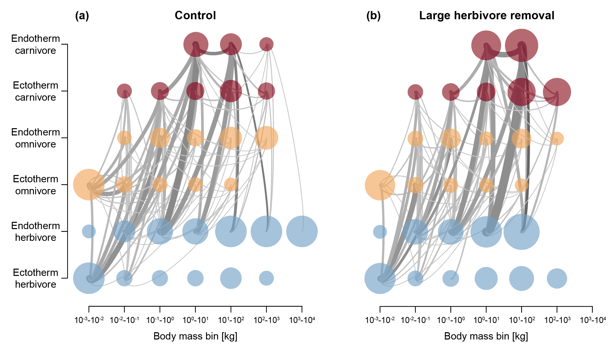
Log10-binned food-web plots constructed from a control simulation (a) and a simulation in which large and mega (>100 kg) endothermic herbivores were removed (b). Node colour depicts feeding category: carnivores (red), omnivores (orange) and herbivores (blue). Grey lines connecting the nodes illustrate the flows between grouped cohorts. These results can be replicated, without any further dependencies, using the code shown in the main text.