Case study 2

In the second example, we reduced the relative biomass of autotrophs (i.e., vegetation) accessible for herbivory and observed how it affected the biomass of endotherms. First a 100-year spin-up simulation was run using the default MadingleyR input parameters. The code below shows how the initialisation and spin-up simulation can be done. Case study one uses the exact same procedure and provides more explanation on the code (see).

library(MadingleyR)

# Set model params
spatial_window = c(31, 35, -5, -1) # region of interest: Serengeti
sptl_inp = madingley_inputs('spatial inputs') # load default inputs

# Initialise model
mdata = madingley_init(spatial_window = spatial_window, spatial_inputs = sptl_inp)

# Run spin-up of 100 years 
mdata2 = madingley_run(madingley_data = mdata,
                       spatial_inputs = sptl_inp,
                       years = 100)

Next, this spin-up simulation is extended by an additional 50 years without any reduction in available autotroph biomass and the end state was used as the control. The 100-year spin-up was then also used to run 8 independent land-use intensity experiments where the fraction accessible stock mass for herbivory was reduced by 0.1 increments to test the effects over a gradient of land-use intensities. This was done by modifying the values of hanpp (human appropriation net primary productivity) spatial input layer and setting apply_hanpp to 1 (apply_hanpp = 1 tells the model to reduce the vegetation using fractional values):

# Set scenario parameters
reps = 5 # set number of replicas per land-use intensity
fractional_veg_production = seq(1.0, 0.1, -0.1) # accessible biomass
fg = c('Herbivore', 'Carnivore', 'Omnivore') # vector for aggregating cohorts
stats = data.frame() # used to store individual model output statistics

# Loop over land-use intensities
for(j in 1:reps){
  
  mdata3 = mdata2 # copy spin-up MadingleyR object to use in replica
  
  for(i in 1:length(fractional_veg_production)) {
  
    print(paste0("rep: ",j," fraction veg reduced: ",fractional_veg_production[i]))
    
    sptl_inp$hanpp[] = fractional_veg_production[i] # lower veg production in the hanpp spatial input layer
    
    mdata4 = madingley_run(
      years = 50,
      madingley_data = mdata3,
      output_timestep = c(99,99,99,99),
      spatial_inputs = sptl_inp,
      silenced = TRUE,
      apply_hanpp = 1) 
    
    # Calculate cohort biomass
    cohorts = mdata4$cohorts
    cohorts$Biomass = cohorts$CohortAbundance * cohorts$IndividualBodyMass
    cohorts = cohorts[cohorts$FunctionalGroupIndex<3, ] # only keep endotherms
    cohorts = aggregate(cohorts$Biomass, by = list(fg[cohorts$FunctionalGroupIndex + 1]), sum)
    stats = rbind(stats, cohorts) # attach aggregated stats
  }
}

The end state of each land-use intensity scenario can then be compared to the control run using the code below:

# Calculate mean relative (to control) response per replica simulation
stats$veg_reduced = rep(sort(rep(1 - fractional_veg_production, 3)),reps)
m = aggregate(stats$x, by = list(stats$veg_reduced, stats$Group.1), FUN = median)
m$x_rel = NA;
for(i in fg) {
  m$x_rel[m$Group.2 == i] = m$x[m$Group.2 == i]/m$x[m$Group.2 == i][1]
}

# Make final plots
plot(1 - unique(fractional_veg_production), m$x_rel[m$Group.2 == 'Herbivore'],
     col= 'green', pch = 19, ylim = c(0, 1.5), xlim = c(0, 1),
     xlab = 'Relative vegetation biomass inaccessible', ylab = 'Relative change in cohort biomass')
points(1 - unique(fractional_veg_production), m$x_rel[m$Group.2 =='Carnivore'], col= 'red', pch = 19)
points(1 - unique(fractional_veg_production), m$x_rel[m$Group.2 == 'Omnivore'], col = 'blue', pch = 19)
abline(1, -1, lty = 2)
legend(0.0, 0.3, fg, col=c('green', 'red', 'blue'), pch = 19, box.lwd = 0)

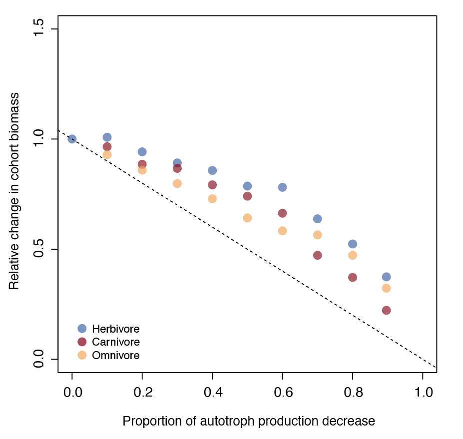
Relative change in biomass of endotherm cohorts compared to the control simulation (biomass experiment/biomass control) plotted against the proportion of plant biomass reduction. A relative change in biomass of 1 indicates no change. Data points represent the relative change in biomass of endothermic carnivores (red), omnivores (orange) and herbivores (blue) averaged over 10 replicas extracted at the end of the 5-year simulation experiment. The dashed line indicates the impact expected if the biomass of endotherms decreased linearly with the amount of plant made inaccessible for feeding (i.e. y = −x).